On dives -whether recreational or technical- if you are using a dive computer, chances are it is running the Bühlmann ZHL-16 Model to keep you safe, as it is one of the most widespread decompression models known today. Its vast documentation, ease of understanding, and easy implementation make it a user-favorite. In this article, I want to talk a little bit about where the ZHL-16 model comes from, what it is, and how it works: in this article, we'll go over some of the mathematical basis for the model as well.
Historically
If you want to learn about the full timeline behind decompression models, we have a full article about the history of decompression models. Here, let's recap how the ZHL-16 specifically came to be.
In the early 20th century, J.S. Haldane developed the first so-called "Haldanian" decompression models, which came in the form of dive tables, telling divers what stops they would have to complete as a function of the depth they went down to (and for how long). These were the first proper decompression schedules published, but although they are now considered the pillar of decompression theory, they were far from optimized. The U.S. Navy was a major player in the further development of decompression models. From the beginning to the end of the 20th century, multiple new tables have been frequently published, based on new research. One issue they had was figuring out a decompression model for ultra-deep and long dives. The U.S. Navy's work culminated in 1965 when Robert D. Workman published his revised tables, taking into consideration the fact that the compartments' supersaturation ratios (more info on that later) could vary as a function of depth.
Starting from 1959, Albert Aloïs Bühlmann would base his work on all the existing decompression theory and the subsequent work from Robert Workman. As Bühlmann was Swiss, he had to take the lower ambient pressure at Swiss lakes into account. The first version of the Bühlmann ZHL model was published in 1983. This version only considered 12 compartments and was appropriately called the ZHL-12.
3 years later, in 1986, Bühlmann would publish his first version of the ZHL-16, with 16 compartments. This first version would come to be known as ZHL-16 A. Later on, some values were slightly adjusted for middle-compartments, and two new versions of this model came to be: the ZHL-16B, created for printing decompression tables, and the ZHL-16C, to be used in Dive computers.
The idea behind the model
The ZHL-16 model, like all Haldanian models, treats the body as composed of parallel "compartments". This means that nitrogen (and more specifically, inert gases in general), instead of diffusing in and out of our body as one block, will saturate and desaturate into and out of each compartment individually. The rate at which inert gas moves into and out (saturation and desaturation) of each compartment will vary; each compartment also has a tolerated saturation pressure that varies with depth. Dive computers and decompression planning software basically track the saturated nitrogen in each compartment and ensure it doesn't exceed the safe limit, and if it does, it imposes mandatory decompression stops (more details on what exactly this safe limit is later).
The gross idea behind the decompression model is the ability to track the inert gas saturation of each compartment individually and ensure none of them surpass the "safe limit". In practice, during the dive, there will be a "leading compartment", which is defined to be the one that is the closest to its safe limit.
Saturation of the Compartments
To calculate the inert gas saturation of the compartments, the ZHL-16 model uses an exponential-exponential gas intake model, following the half-times of each compartment. This means that after one half-time, the compartment will be 50% saturated, after two half-times, it will be 75% saturated, after three half-times, 87.5% saturated, etc... The graphs underneath illustrate a compartment with a 5-minute half-time saturating and desaturating over time.
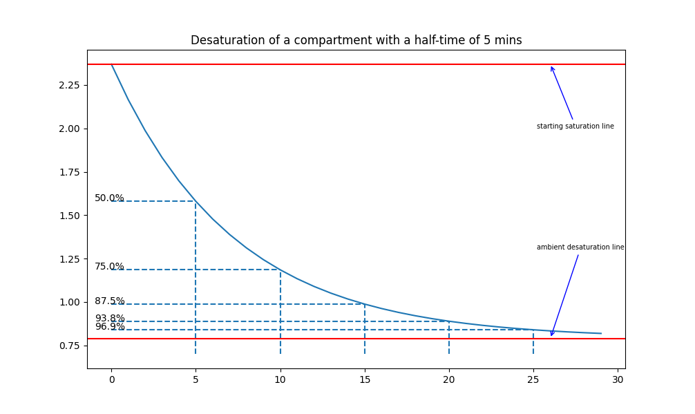
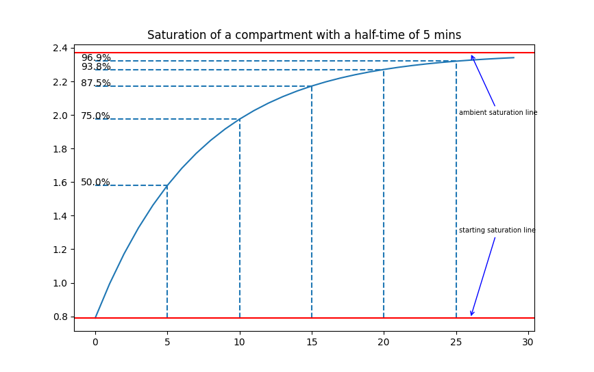
Examples of desaturation/saturation in a compartment with a half-time of 5 minutes.
The exchange of gas between alveolar gas and each compartment is described by the following differential equation:
\[ \frac{dp_i}{dt}=k_i(p_{alv}(t)-dp_i) \]With ki being a constant depending on each compartment's half-time. Solving this differential equation will yield two different forms depending on whether the alveolar pressure is constant (if the diver is stationary) or varying linearly with depth (if the diver descends or ascends with a constant speed). In the case of constant alveolar pressure, we will have the famous Haldane equation:
\[ p_i(t) = p_{alv} + (p_i(0)-p_{alv})\cdot e^{-k_it} \]In the case of a variable alveolar pressure (considering the diver is moving at a constant rate r), solving the differential equation will give us the Schreiner equation:
\[ p_i(t)=p_{alv}(0)+Q(t-\frac{1}{k_i})-(p_{alv}(0)-p_i(0)-\frac{Q}{k_i})e^{-k_it} \]We can define ki = ln(2)/t1/2 with t1/2 being the half-time of the compartment in question, and Q the rate of change of the inspired inert gas fraction.
By using those two equations, the ambient pressure, and the inspired inert gas fraction, this model allows us to compute the dissolved inert gas in each compartment. If you are interested in how those two equations were found, read about how to find the Haldane and Schreiner equations. The alveolar inert gas pressure used in the equation slightly differs from the inspired inert gas pressure (due to the presence of saturated water vapor and carbon dioxide): read this to learn how to calculate the alveolar pressure of inert gas.
Each compartment will have to be calculated independently. Additionally, if there are multiple inert gases to take into consideration (e.g., a trimix blend containing helium on top of nitrogen), each inert gas will have to be calculated separately. To accurately track the inert gas amount in our tissues, each step of the dive plan will have to be separated and considered as static (in which case the Haldane equation will be used) or dynamic (in which case the Schreiner equation will be used).
M-values
Now that we are able to calculate the inert gas saturation of our tissues, the next step in this model is calculating the tolerated saturation levels of each of those tissues, also called M-values.
M-values (whose unit is pressure) represent the amount of pressure tolerated by each compartment at a specific ambient pressure. Each compartment is given two coefficients, called a and b, which are used to calculate this tolerated pressure. To be more precise, the original work from Bühlmann provides a formula to calculate the tolerated ambient pressure as a function of tissue tension:
\[ P_{amb.tol} =(P_{i.g.t}-a) ·b \]This formula can be rearranged to calculate the tolerated tissue tension as a function of ambient pressure:
\[ P_{i.g.t} =\frac{P_{amb.tol}}{b} + a \]The a and b values for each compartment vary with versions of the model: as explained previously, the Bühlman ZHL model has had several versions, with the most accepted one still widely in use to this day being the ZHL-16C. The coefficients of this model are as follows:
compartment |
1 | 2 | 3 | 4 | 5 | 6 | 7 | 8 | 9 | 10 | 11 | 12 | 13 | 14 | 15 | 16 |
|---|---|---|---|---|---|---|---|---|---|---|---|---|---|---|---|---|
half-time (min) Nitrogen |
5.0 | 8.0 | 12.5 | 18.5 | 27.0 | 38.3 | 54.3 | 77.0 | 109.0 | 146.0 | 187.0 | 239.0 | 305.0 | 390.0 | 498.0 | 635.0 |
a Nitrogen |
1.1696 | 1.0 | 0.8616 | 0.7562 | 0.62 | 0.5043 | 0.441 | 0.4 | 0.375 | 0.35 | 0.3295 | 0.3065 | 0.2835 | 0.261 | 0.248 | 0.2327 |
b Nitrogen |
0.5578 | 0.6514 | 0.7222 | 0.7825 | 0.8126 | 0.8434 | 0.8693 | 0.8910 | 0.9092 | 0.9222 | 0.9319 | 0.9403 | 0.9477 | 0.9544 | 0.9602 | 0.9653 |
half-time (min) Helium |
1.88 | 3.02 | 4.72 | 6.99 | 10.21 | 14.48 | 20.53 | 29.11 | 41.20 | 55.19 | 70.69 | 90.34 | 115.29 | 147.45 | 188.24 | 240.03 |
a Helium |
1.6189 | 1.383 | 1.1919 | 1.0458 | 0.922 | 0.8205 | 0.7305 | 0.6502 | 0.595 | 0.5545 | 0.5333 | 0.5189 | 0.5181 | 0.5176 | 0.5172 | 0.5119 |
b Helium |
0.4770 | 0.5747 | 0.6527 | 0.7223 | 0.7582 | 0.7957 | 0.8279 | 0.8553 | 0.8757 | 0.8903 | 0.8997 | 0.9073 | 0.9122 | 0.9171 | 0.9217 | 0.9267 |
Notice the half-times and a/b values for nitrogen and helium are different. If both are present in the diver's tissue, the total inert gas amount should be considered (sum of nitrogen and helium), and a new value for a and b should be calculated using a weighted average:
\[ a = \frac{p_{i,N_2}a_{N_2}+p_{i,He}a_{He}}{p_{i,N_2}+p_{i,He}} \] \[ b = \frac{p_{i,N_2}b_{N_2}+p_{i,He}b_{He}}{p_{i,N_2}+p_{i,He}} \]As the tolerated tissue tension is directly proportional to ambient depth, the intuitive way to think about it is that the tolerated inert gas tissue tension increases the deeper one goes, and as the diver shallows up, this tolerance decreases. When ascending from a decompression dive, a decompression model would need to ensure none of the M-value lines are exceeded. In the ZHL-16C model, this means constantly comparing the tissue tensions of each of the 16 compartments to their associated M-value line. To illustrate, the graph below shows a representation of the 16 nitrogen lines in the ZHL-16C model:
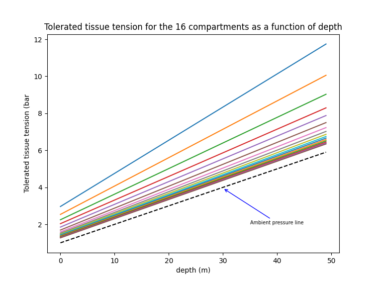
The faster tissues have a higher tolerance compared to the slow tissues. This means they can have a greater supersaturation level. This has multiple consequences: the faster compartments will be limiting factors for short dives (because even though their tolerance are higher, they saturate faster and reach their limit faster), but upon ascending and off-gassing those faster tissues, the slower tissues will still be on-gassing towards their M-value limit. This also begs the question of the viability of deep stops regarding deep tissue saturation.
An important point to keep in mind is what M-values or M-value lines represent: the "maximum tolerated tissue tension" is a very grey area and varies from person to person (the tolerance can vary with age, fitness level, leanness, hydration levels, and many other factors). M-values are a mathematical tool that attempts to create a solid boundary within this grey area. The numerical value this boundary gives us is an average gathered over many dives.
If you are interested, you can read this article to learn more about M-values.
Gradient Factors
Gradient Factors allow us to control the conservatism of our decompression profile. As explained previously, M-values represent a theoretical line that shouldn't be crossed at any point to avoid DCI risks. It then follows that during their ascent, the diver will attempt to stay away from this theoretical line as much as possible. However, being too conservative will also lead to unoptimal off-gassing. The Bühlmann ZHL models introduce two numbers known as gradient factors, represented as X/Y, with X representing GF Low, and Y representing GF High; both of these numbers represent (in percentages) how close to the M-value line the diver will be allowed to be during his ascent.
- The GF Low controls the first stop: this means that once a tissue gets to the chosen percentage of the M-value line, a stop will be generated and the decompression will start.
- The GF High controls the surface gradient: this means that the most saturated tissue will have to be below this chosen percentage of its M-value to be allowed to surface and end the dive.
Examples of common gradient factors include 40/80, 50/85, 70/70, but the "perfect" gradient factor is a constant ongoing debate between divers (and, at the end of the day, mostly comes down to personal preferences).
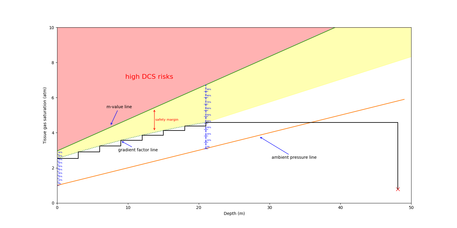
Gradient factors will act as a ramp and bring the diver from the Low gradient factor to the high gradient factor over the ascent. Knowing the depth of the first decompression stop, intermediate gradient factor values can be calculated as follows:
\[ GF_{depth}=GF_{HIGH}-\frac{GF_{HIGH}-GF_{LOW}}{DEPTH_{First stop}}\cdot DEPTH_{current} \]The following image illustrates how gradient factors work and allow us to decompress while staying away from the M-value line. Keep in mind, in the illustration, only one compartment is shown for the sake of simplicity; in a real decompression software, all of the 16 compartments will have to be verified simultaneously.
For a more in-depth explanation of the topic, you can read this article about Gradient Factors.
The model in action
Tissue saturation/desaturation, M-values, and gradient factors constitute the bread and butter of the ZHL-16 models, but in practice, how do decompression software use all of that to generate a decompression plan? Assuming a diver is using a given gas blend (and ignoring separate issues such as decompression gas blends), this is how a decompression plan can be generated:
- The bottom plan (including the depth, time at depth, and gas mix) is given to the decompression software. The saturation is calculated upon descent and during the stop at the planned depth.
- A grid of "depth intervals" is chosen, along which the diver will have to perform eventual decompression stops (the most common depth intervals decompression divers use are multiples of 3's, i.e., 0m, 3m, 6m, 9m, 12m, etc...).
- Go from the current depth to the next depth along that "depth grid" and verify if any compartment has a higher tissue tension than its associated M-value (taking gradient factors into account).
- If it is the case, go back to the previous depth and add a unit of time (1 minute, for example) to decompress, and re-calculate all tissue saturation levels. Go back to the previous step (3).
- If all compartments do not exceed their GF-weighted M-values, validate the ascent to the next depth along the grid, and repeat the process from step (3).
- Repeat those steps until the diver is back at the surface. This will yield a list of times required at each depth to decompress appropriately
In a dive computer, the concept is similar, the difference being that all nitrogen loading is more accurate due to it being able to monitor depth in real time. Additionally, rather than calculate the current allowed tissue supersaturation as a function of ambient pressure, the computer will calculate the minimum allowed ambient pressure as a function of tissue tensions (and adequately provide the depth ceiling).