On optimizing the safety stop for recreational dives

Introduction

On recreational dives, a safety stop is a non-mandatory stop done at the end of a dive to give more time to the tissues to off-gas the excess nitrogen, giving divers an extra margin of safety. Although varying between each agency and each dive center, it is usual for safety stops to take place at a depth of 5 meters for 3 minutes (a depth of 6 meters isn't uncommon either).

Although they are non-mandatory, they have been shown to decrease silent bubble occurrences (a precursor to Decompression Sickness) and increase safety for successive dives.

In this article, I will first show how a safety stop affects the nitrogen level in your body (I will use the ZH-L16C model which makes us track the nitrogen level in 16 distinct body compartments, but more on that later), then, try to hypothesize alternative safety stops, by varying the time and the depth, and attempt to find a safety stop that maximizes nitrogen off-gassing.

As a side note, it is important to understand that the standard safety stop at 5 meters for 3 minutes is generally good for beginners as it is easy to maintain: although I may find a more "ideal" safety stop in terms of inert gas offloading, those may be harder for novice divers to follow accurately, and therefore I wouldn't necessarily recommend to anyone to switch to a different safety stop protocol.

Methodology

The objective of this part is to explain the exact process -from the theory to the implementation of the code- to understand how I am able to get the results that I do.

model used

To model inert gas de/saturation in our body, I will use Bülhmann's compartmental model: ZH-L16C, combined with the Haldane equation (1) and the Schreiner equation (2) (detailed below), to respectively calculate the inert gas de/saturation at rest and at constant pressure change (meaning ascending and descending at a constant speed)

\[P_{I,\text{ig}}(t_e) = P_{I,\text{ig}}(t_0) + (P_{gas,ig} - P_{I,\text{ig}}(t_0)) \cdot (1 - 2^{-t_e \over t_{I, 1/2}}) \quad (1)\] \[P_{I,\text{ig}}(t_e) = P_{gas,ig} + R \cdot (t_e - {t_{I, 1/2} \over {\ln 2}}) - (P_{gas,ig} - P_{I,\text{ig}}(t_0) - {{R \cdot t_{I, 1/2}} \over {\ln 2}}) \cdot 2^{-t_e \over t_{I, 1/2}} \quad (2)\] \( P_{I,\text{ig}}(t_e): \text{Partial pressure of the inert gas dissolved in the compartment I} \\ \text{at the end of the exposure, expressed in bar} \) \(P_{I,\text{ig}}(t_0): \text{Partial pressure of the inert gas dissolved in the compartment I} \\ \text{before the exposure, expressed in bar} \) \(P_{gas,ig}: \text{Partial pressure of the inert gas in the breathing mix at ambient} \\ \text{pressure, expressed in bar} \) \(t_e: \text{duration of exposure, expressed in minutes}\) \(t_{I, 1/2}: \text{half time of the compartment I, expressed in minutes}\) \(R: \text{rate of change of the partial pressure of the inert gas in the} \\ \text{breathing mix, expressed in bar/min}\)

The ZH-L16C model splits the body into 16 different compartments, each representing different tissues, from the most perfused ones to the least perfused ones: essentially, the lower number compartments in-gas and off-gas faster than the highest number compartments; this is represented by a respectively lower and higher half-time, which represents the time it takes for a certain tissue to in-gas half of its maximum saturation value. The model gives us a tool to find the maximum dissolved inert gas partial pressure allowed for each compartment: there are two coefficients for each compartment, called a and b, which can be used to calculate the maximum tolerated saturation level for a certain ambient pressure according to the following formula (3):

\[P_{I,\text{tol}} = {P_{amb} \over b} + a \quad (3)\]

The ZH-L16 model has three different tables for a values: tables A, B, and C. As C uses the most conservative values for calculating the tolerated pressure, I will use it to calculate each compartment's M-value and will refer to the ZH-L16 model as the ZH-L16C.

compartment nb	1	2	3	4	5	6	7	8	9	10	11	12	13	14	15	16
half-time (min)	5.0	8.0	12.5	18.5	27.0	38.3	54.3	77.0	109.0	146.0	187.0	239.0	305.0	390.0	498.0	635.0
a	1.1696	1.0	0.8616	0.7562	0.62	0.5043	0.441	0.4	0.375	0.35	0.3295	0.3065	0.2835	0.261	0.248	0.2327
b	0.5578	0.6514	0.7222	0.7825	0.8126	0.8434	0.8693	0.8910	0.9092	0.9222	0.9319	0.9403	0.9477	0.9544	0.9602	0.9653
ptol at 1 atm (bar)	2.962	2.535	2.246	2.034	1.851	1.690	1.591	1.522	1.475	1.434	1.403	1.370	1.339	1.309	1.289	1.269

I will compare each compartment's saturation level to its maximum allowed value and observe how each simulated safety stop affects each compartment's inert gas level.

defining recreational dives

In this context, I will define recreational dives as dives not requiring any mandatory decompression stop to ascend during any point in the dive. Meaning, the dissolved inert gas in each compartment never exceeds the maximum tolerated value of each individual compartment at the surface pressure. More rigorously, we could describe it as:

\( P_{I,\text{ig}}(t) < P_{I,\text{tol}}(P_{amb}=1) \quad \forall {t,I} \)

Of course, the safety stop does not count as a mandatory decompression stop.

Diving operations & nitrogen values

To visualize each compartment's nitrogen level (which I will call "nitrogen values" interchangeably), I will call each compartment C_i, i being a number between 1 and 16. I will then call C_1,16 the tuple containing all compartments.

\(C_{1,16} = (C_1, C_2, C_3, \dots, C_{16}) \)

An "operation" on a compartment (a tissue) is defined as a duration over which the nitrogen value of said tissue changes. Examples of "operations" include compression at depth during a bottom time (on-gassing), deco & safety stops (off-gassing), ascents & descents (mix of on and off-gassing). An operation that takes place at a constant depth, such as a deco stop or a bottom time will be modeled using the Haldane equation. An operation where the depth varies (ascents & descents) will be modeled using the Schreiner equation.

As all operations affect all compartments at the same time, varying only by the different half-time for each compartment, it is important to understand that while each operation will be applied to the tuple as a whole, it will modify each compartment's nitrogen value individually.

A succession of operations on the compartments could be represented as follows: (the relevant equation used is shown on top of the arrow).

\( C^1_{1,16} \xrightarrow[\text{bottom time}]{\text{haldane's eq}} C^2_{1,16} \xrightarrow[\text{ascent}]{\text{Schreiner's eq}} C^3_{1,16} \xrightarrow[\text{safety stop}]{\text{haldane's eq}} C^4_{1,16} \)

After each operation, as the nitrogen content of each tissue will vary, we can plot the nitrogen partial pressure as a function of each compartment to visualize it. Before explaining the code behind it, the following graph is the one we want to obtain (figure 1)

In this scenario, the diver is breathing a mix of 21% Oxygen 79% (Air) and completes a bottom time of 10 minutes at 30m, before slowly ascending at a 5m/min rate up to a depth 5m, where he completes a 3-minute safety stop, where he then exits the water

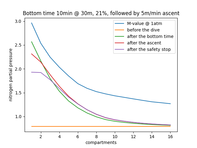
You will notice that I take the ascent into account but not the descent: that is because if I were to plan a dive, I would include the descent into the bottom time, this adds a small layer of safety as we are slightly overestimating how much the body on-gasses. The final ascent from the safety stop to the surface is also not taken into account, but more on that later as the final ascent speed will be an important point.

Normalized tissue saturation/Surface gradient

Another way of visualizing the amount of nitrogen in each tissue is to "normalize" it: we divide the nitrogen partial pressure by the surface M-value of each tissue. I will call this ratio \(C_{norm,I}\) (\(I\) being a number between 1 and 16 representing a certain compartment) and define it as:

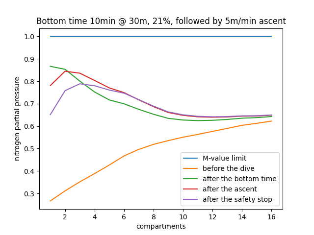
\[C_{norm,I} = {C_I \over P_{I,\text{tol}}(P_{amb} = 1)} \quad (4)\]

For a certain tissue, when \(C_{norm,I} = 1\), that means that the tissue is exactly at its surface M-value. when \(C_{norm,I} > 1\), the tissue is above its surface M-value (in which case the diver cannot directly ascend and will need to do decompression stops before), and if \(C_{norm,I} < 1\), the tissue is below its M-value. If all tissues are below 1 (\(C_{norm,I} <1, \forall I\)), the diver is within recreational limits, but the closer \(C_{norm,I}\) comes to 1 for a certain tissue, the closer the tissue is to its M-value, and therefore it is in our best interest to minimize it. Applying this to the previous graph, the normalized curves would look as follows (figure 2):

Code

This part is purely about explaining the code used to model the compartments, it is quite extensive and helps to understand how I get the graphs & results, but it is not completely required to read it to interpret and understand the results, so if you're not a coding person, feel free to skip this part.

The full code is available and free to download below

My idea was to group all tissue compartments in a class, from which I could obtain the nitrogen partial pressure value of each tissue at any time, modify it through "operations" (specified before), using the Haldane or Schreiner equation, and then plot all those values, "Normalized" or not. Have a look at it and I will detail each part further down:

import matplotlib.pyplot as plt
import math as m


def haldane(pressure_0, exposure_time, half_time, breathing_mix_ambient):
    """
    returns the inert gas saturation value of a specific tissue exposed to a gas mix at a certain depth after a certain time
    variable breathing_mix should reflect the nitrogen partial pressure of the mix AT THE BREATHED DEPTH
    """
    return (pressure_0 
    + (breathing_mix_ambient - pressure_0)
    *(1-2**(-exposure_time/half_time)))
    
def schreiner(pressure_0, exposure_time, half_time, breathing_mix_ambient, R):
    """
    incorporates a constant ascent or descent speed into the haldane equation
    the variable represents the change in pressure/min:
    R = rate * gas fraction
    -for an ascent of 10m/min, rate=-1
    -for a descent of 10m/min, rate=1
    """
    return (breathing_mix_ambient 
            + R*(exposure_time - half_time/m.log(2)) 
            - (breathing_mix_ambient - pressure_0 - R*half_time/m.log(2))
            *2**(-exposure_time/half_time))

class ZH_L16C:

    def __init__(self):
        
        #compartment nb: N2 partial pressure, t1/2, a, b
        #Do NOT modify those values, use the lists below, this dic is only used to initialise list values
        self.compartments = {1: [0.79, 5.0, 1.1696, 0.5578],
            2: [0.79, 8.0, 1.0, 0.6514],
            3: [0.79, 12.5, 0.8616, 0.7222],
            4: [0.79, 18.5, 0.7562, 0.7825],
            5: [0.79, 27.0, 0.62, 0.8126],
            6: [0.79, 38.3, 0.5043, 0.8434],
            7: [0.79, 54.3, 0.441, 0.8693],
            8: [0.79, 77.0, 0.4, 0.8910],
            9: [0.79, 109.0, 0.375, 0.9092],
            10: [0.79, 146.0, 0.35, 0.9222],
            11: [0.79, 187.0, 0.3295, 0.9319],
            12: [0.79, 239.0, 0.3065, 0.9403],
            13: [0.79, 305.0, 0.2835, 0.9477],
            14: [0.79, 390.0, 0.261, 0.9544],
            15: [0.79, 498.0, 0.248, 0.9602],
            16: [0.79, 635.0, 0.2327, 0.9653]}
            
        #Used to modify and track the nitrogen level of tissues
        self.compartment_N2 = [self.compartments[i+1][0] for i in range(len(self.compartments))]
        
        #Do not modify, use for manipulating
        self.compartment_half_time = [self.compartments[i+1][1] for i in range(len(self.compartments))]
        self.compartment_a = [self.compartments[i+1][2] for i in range(len(self.compartments))]
        self.compartment_b = [self.compartments[i+1][3] for i in range(len(self.compartments))]
     
    def haldane(self, exposure_time, depth, O2_mix, modify=True):
        """
        Modifies the compartments nitrogen level according to haldane's equation
        This supposes a static excposure at a certain depth
        """
        breathing_mix = (1-O2_mix)*(1+depth/10)
        new_values = [haldane(self.compartment_N2[i], exposure_time, self.compartment_half_time[i], breathing_mix) for i in range(len(self.compartments))]
        
        if modify:
            self.compartment_N2 = new_values
            
        return new_values
        
    def schreiner(self, exposure_time, start_depth, end_depth, O2_mix, modify=True):
        """
        incorporates shreiner's equation in the model class, modifying compartment nitrogen level based
        on a constant ascent/descent
        """
        breathing_mix = (1-O2_mix)*(1+start_depth/10)
        rate = (end_depth-start_depth)/(exposure_time*10)
        new_values = [schreiner(self.compartment_N2[i], exposure_time, self.compartment_half_time[i], breathing_mix, rate*(1-O2_mix)) for i in range(len(self.compartments))]
        
        if modify:
            self.compartment_N2 = new_values
            
        return new_values
        
    def M_values(self, Pamb = 1):
        """
        Calculates the maximum tolerated N2 saturation for a certain ambient pressure
        """
        return [self.compartment_a[i]+Pamb/self.compartment_b[i] for i in range(len(self.compartments))]
        
    def plot_M(self, Pamb = 1):
        """
        plots the M-value of each tissue for a certain ambiant pressure
        """
        x_axis = [i+1 for i in range(len(self.compartments))]
        y_axis = self.M_values(Pamb = Pamb)
        plt.plot(x_axis, y_axis, label="M-value @ {Pamb}atm".format(Pamb=Pamb))
    
    
    def plot_N2(self, label="Nitrogen tissue level"):
        """
        plots all nitrogen partial pressure (in bar) as a function of each compartment
        """
        x_axis = [i+1 for i in range(len(self.compartments))]
        plt.plot(x_axis, self.compartment_N2, label=label)
        
    def plot_N2_M_ratio(self, label="Ptissue/M-value"):
        """
        plots the ratio of each compartments nitrogen partial pressure to its M-value
        A 1 on the graph means that the tissue is at its M-value
        """
        x_axis = [i+1 for i in range(len(self.compartments))]
        M_values = self.M_values(Pamb = 1)
        ratio_N2_M = [self.compartment_N2[i]/M_values[i] for i in range(len(self.compartments))]
        plt.plot(x_axis, ratio_N2_M, label=label)

That is quite a lot to read at once so let's break it down step by step:

__init__() function: Creates the variables such as the nitrogen level inherent to each model instance. By calling model.compartment_N2[0], we are able to access the nitrogen level of the first compartment (as the list index starts at 0, not 1). Similarly, self.compartment_half_time, self.compartment_a, self.compartment_b contains each tissue's half-time, a-values, and b-values(which are then used to calculate the M-values and in on-off gassing models).

haldane() function: Modifies the nitrogen level of compartment_N2 according to a constant-depth on/off-gassing model. For instance, if we want to simulate a bottom time of 10 minutes at 30m breathing air, we would call model.haldane(10, 30, 0.21). It uses the value of compartment_N2 before the function call as the initial nitrogen value.

schreiner() function: Similarly to the haldane() function, the schreiner() function modifies the nitrogen level of compartment_N2, but it is based on a constant ascend/descend speed instead of assuming a constant depth. Needs to be called by passing the initial depth, final depth, and time of ascent/descent as arguments. For instance, if we want to simulate an ascent from 40m to 5m in 10 minutes while breathing air, we would call model.schreiner(10, 40, 5, 0.21).

M_values() function: Takes the ambient pressure as an argument and returns the M-value of all tissues at that pressure.

plot_M() function: Takes the ambient pressure as an argument and plots the associated M-values (for all compartments).

plot_N2() function: This function plots the current nitrogen level of each compartment.

plot_N2_M_ratio() function: plots the ratio of nitrogen level to the M-level of each compartment, creates "normalized" graphs that I explained previously.

Using that class makes it easy to manipulate our theoretical diver: if we want to obtain both previous graphs, we now simply have to write the following for Figure 1:

def main():
    model = ZH_L16C()
    
    model.plot_M(Pamb = 1)
    model.plot_N2(label="before the dive")
    
    model.haldane(10, 30, 0.21) #10 minutes, 30 meters, breathing 21% O2
    model.plot_N2(label="after the bottom time")
    
    model.schreiner(5, 30, 5, 0.21) #5 minutes to ascend from 30m to 5m, breathing 21% O2
    model.plot_N2(label="after the ascent")
    
    model.haldane(3, 5, 0.21) #3 minutes at 5 meters, breathing 21% O2
    model.plot_N2(label="after the safety stop")
    
    plt.title("Bottom time 10min @ 30m, 21%, followed by 5m/min ascent")
    plt.legend()
    plt.xlabel("compartments")
    plt.ylabel("nitrogen partial pressure")
    plt.show()
   

if __name__ == "__main__":
    main()

And if we want to visualize the "normalized" graph instead (Figure 2), the code can slightly be altered to:

def main():
    model = ZH_L16C()
    
    #following line plots a horizontal line showing the M-value limit
    plt.plot([i+1 for i in range(len(model.compartments))], [1 for i in range(len(model.compartments))], label="M-value limit")
    model.plot_N2_M_ratio(label="before the dive")
    
    model.haldane(10, 30, 0.21) #10 minutes, 30 meters, breathing 21% O2
    model.plot_N2_M_ratio(label="after the bottom time")
    
    model.schreiner(5, 30, 5, 0.21) #5 minutes to ascend from 30m to 5m, breathing 21% O2
    model.plot_N2_M_ratio(label="after the ascent")
    
    model.haldane(3, 5, 0.21) #3 minutes at 5 meters, breathing 21% O2
    model.plot_N2_M_ratio(label="after the safety stop")
    
    plt.title("Bottom time 10min @ 30m, 21%, followed by 5m/min ascent")
    plt.legend()
    plt.xlabel("compartments")
    plt.ylabel("nitrogen partial pressure")
    plt.show()
   

if __name__ == "__main__":
    main()

Putting the model into practice

Now that we know how to graph nitrogen levels after certain dive profiles, I want to graph how different safety stops will affect different dive profiles. To start, there will be 4 different scenarios on which the tissue on-gassing will be calculated:

• A bottom time of 10 minutes at 40m, breathing air
• A bottom time of 10 minutes at 30m, breathing air
• A bottom time of 10 minutes at 30m, breathing air
• A bottom time of 10 minutes at 30m, breathing air

After the bottom time, in all those scenarios, the diver will ascend at a rate of 10m/minute to a depth of 5m, where he will then perform one of the following safety stop plan:

• No safety stop
• 3 minutes at 5 meters
• 2 minutes at 5 meters followed by 2 minutes at 3 meters
• 1 minute each meter from 5 to 1 meter (5 and 1 included)

We will then get a total of 16 curves (4 different safety stops for 4 different scenarios). Of course, some safety stops are longer than others which might skew the result in its favor, but to start, it is good to be able to visualize the results. I chose to graph the "normalized" curves (meaning that for each tissue, I divide its nitrogen level by its M-value).

Note: from now on, although I modify slightly the code to plot multiple graphs at the same time or change a few other things, I will refrain from talking about the code to focus on the theory behind it.

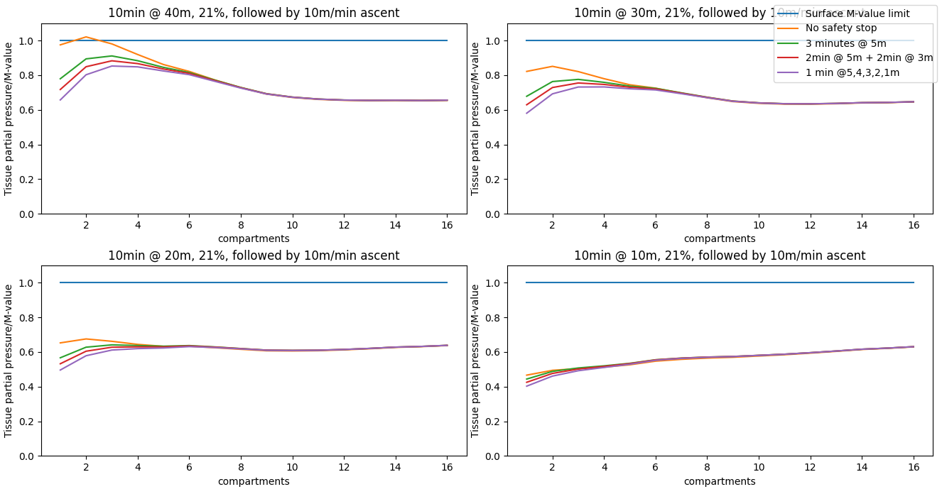
We can observe that for the first few compartments (meaning, the compartments with the lowest half-time and the highest M-values), the longer the safety stop, the better, and at first glance, it does look like separating the safety stop into multiple smaller stops, does help off-gas. However, before concluding anything, let's look at what happens for the last compartments (highest half-time and lowest M-values).

It looks like the nitrogen level of the last compartments blur in together, and it is a bit hard to see what exactly is going on, so let's zoom in and focus on them.

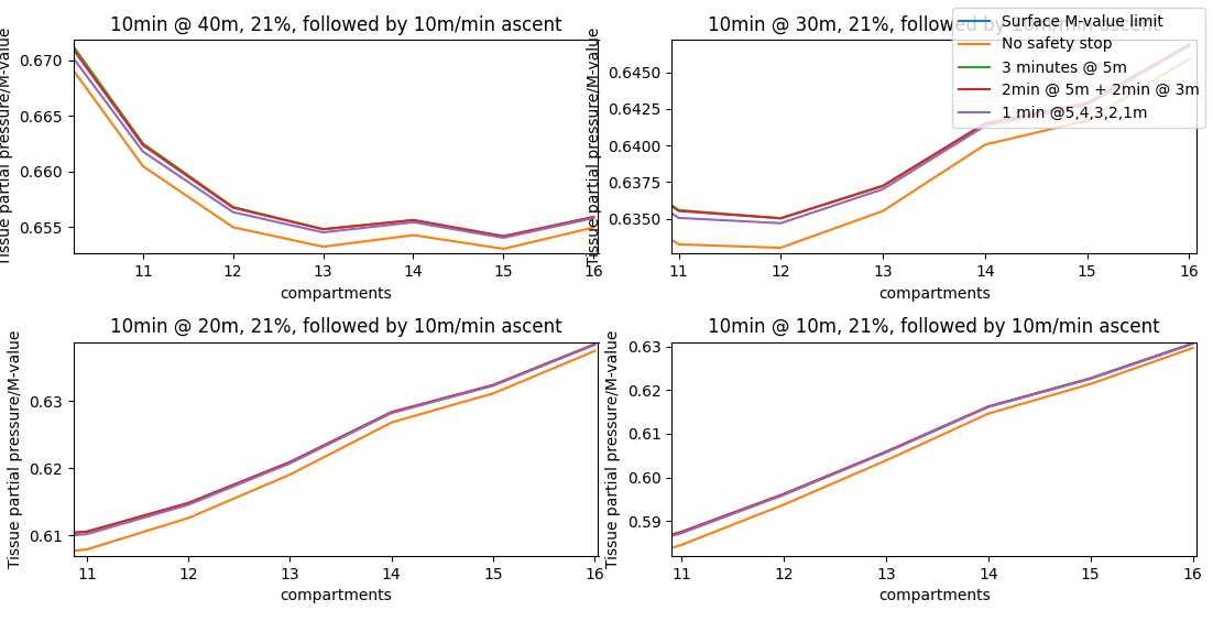
We can observe that for those last compartments, the opposite is true: in the scenario where there are no safety stops, those compartments have a lower nitrogen saturation upon surfacing. Intuitively, we can imagine that during the bottom time, those last compartments will saturate more slowly due to their higher half-time. Being in a recreational setting, we are not staying deep for a significant amount of time, meaning that when we shallow up, those compartments will still be "on-gassing" while completing the safety stop, while the first compartments have already begun to off-gas.

Going further

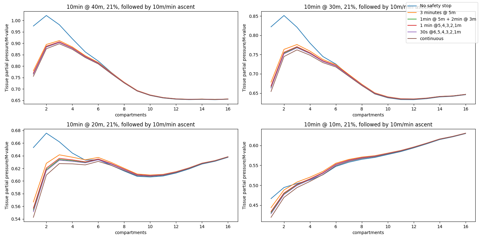
There is a trend appearing on the previous graphs: the more gradual a safety stop is, the lower the nitrogen saturation upon surfacing. The issue with the previous results is that the different safety stops had different durations (which might skew the result a little bit), so we will change it as to have every stop last 3 minutes, but making them as gradual as possible. We will once again have 4 different scenarios (10 minutes at 40m, 30m, 20m, 10m while breathing air), with the following stops:

• 3 minutes static at 5 meters
• 1 minute at 5 meters, followed by 2 minutes at 3 meters
• 1 minute at 5, 4, and 3 meters respectively
• 30 seconds at 6, 5, 4, 3, 2, and 1 meters respectively
• constant ascent speed from 6m to the surface over 3 minutes

The code to obtain the graphs above is available below:

Although it is a bit tricky to see, in all scenarios, the more continuous the safety stop is, the lower the nitrogen level is upon surfacing. Even in the tissues with the higher half-times, the continuous safety stop minimizes the on-gassing at shallower depths!

That being said, there is a line to be found between the optimal safety stop in theory and the optimal safety stop in practice: even though a simple static stop at 5 meters isn't as optimal as others, in practice, it is very easy to carry out; same as the "optimized" slow continuous ascend: although it's great on paper, it is significantly harder to carry out in practice!