Decompression theory is a fascinating subject, as it is a branch that combines physiology, physics, and mathematics to create a model of how inert gases behave in the body, allowing us to understand how to safely conduct a dive without getting DCS (or the bends). Decompression planning software allows divers to input their target depth, bottom time, and available gases; in return, it outputs a decompression table, which, according to certain parameters (which we will discuss later), tells the diver which decompression stops to complete in order to return safely to the surface. What I want to tackle in this article is what happens behind the curtains; what does the decompression software exactly do between getting the initial bottom plan and returning the full decompression table?
As the first version of our decompression planner was published recently, writing an article about how such a tool works is a double opportunity: first of all, we believe it's a good thing to talk about decompression theory and create more knowledgeable divers, but secondly, it also serves as a way to be transparent about the logic behind our own software and ensure nothing is left to the imagination of the user. In this article, I will try to talk about decompression theory as much as I talk about the implementation of it in the model, although it is important to keep in mind that every software can slightly differ in its implementation.
Buckle in and get ready to dive deep into the mechanisms of decompression models!
Validating user input - A preface
Before delving into the actual juicy parts of the math, M-values, gradient factors, and everything else, I wanted to mention the user input issue. As you will see later on, creating a decompression planning software comes with a lot of variables, which are used for various reasons (such as configuring the environment to compute the pressure or choosing the conservatism of the model). Some of the variables shouldn't be modifiable by the user (such as the gravitational acceleration of Earth, unless we want to generate a decompression plan on another planet), but some variables definitely should be. For example, to have an accurate decompression plan, the user should be allowed to input their Altitude, the water density (salinity), or even their gases. The issue occurs when the user inputs a completely invalid entry, and risks messing up the decompression plan - for example, inputting a water density that is too low will lead to the model computing a lower pressure at a certain depth, which will yield an inadequate decompression plan. For that reason, it is important to verify that the values the user inputs are reasonable (and prevent the model from running if any aren't). For our decompression planner, we implemented the following conditions:
- Altitude must be between 0m and 10000m
- Water density must be between 990 kg/m^3 and 1055 kg/m^3
- Pressure at sea level must be between 95 kPa and 105 kPa
- Ascent & Descent rate must be between 1m/s and 50m/s
- The gas used must have at least 1% Oxygen, and the Helium percentage plus Oxygen percentage should be between 1-100%
- Depths and times must be integers and non-negative.
If all values are acceptable, then the model can be allowed to run!
Building a Pressure Engine
The first crucial step to allow our model to work properly is being able to calculate the real pressure at any depth. When first learning about diving and pressure, we are usually told "the pressure increases at a rate of 1 atmosphere every 10 meters (or 33 feet)". Taking the surface pressure of 1 atmosphere into account, we get an approximation formula for the pressure:
\(P = D/10+1\) \(\text{Where D is the depth in meters.}\)However, for a full-fledged decompression planner, this isn't good enough: we don't want an approximation that can potentially accumulate errors and yield a bad (or even dangerous) decompression plan. We'll need to be able to compute the pressure for any depth as accurately as possible, and to do that, we're going to calculate the hydrostatic pressure in the water column by using the following formula:
\(p(z) = \rho g z + p_{surf}\) \( p(z): \text{Pressure at depth z (in } Pascal) \) \( \rho : \text{Water density (in }kg/m^3) \) \( g : \text{Gravitational acceleration (on earth, }g\simeq 9.81m/s^2) \) \( z : \text{Water depth (in }m) \) \(p_{surf}: \text{Pressure at surface (in }Pascal)\)One thing to notice is that in the realm of diving, we usually talk about pressure in units of bar or atmospheres, but for calculating in the SI system, pressure is expressed in Pascal (Pa), where 1 bar = 100,000Pa. The second thing to notice is that water density will depend on where the user is diving; in freshwater, it is around 1000kg/m^3, while saltwater can have a water density ranging from 1020 to 1050 kg/m^3. In our decompression planner, the water density -if left unchanged- is at 1025kg/m^3 by default.
Something else to take into account is the surface pressure. As said previously, we usually approximate the surface pressure to 1 bar, but if we want to be more accurate, we will have to calculate it as a function of altitude: At sea-level (0m altitude), the pressure is on average 101.3kPa, or 1.013 bar, and it decreases as we go higher:
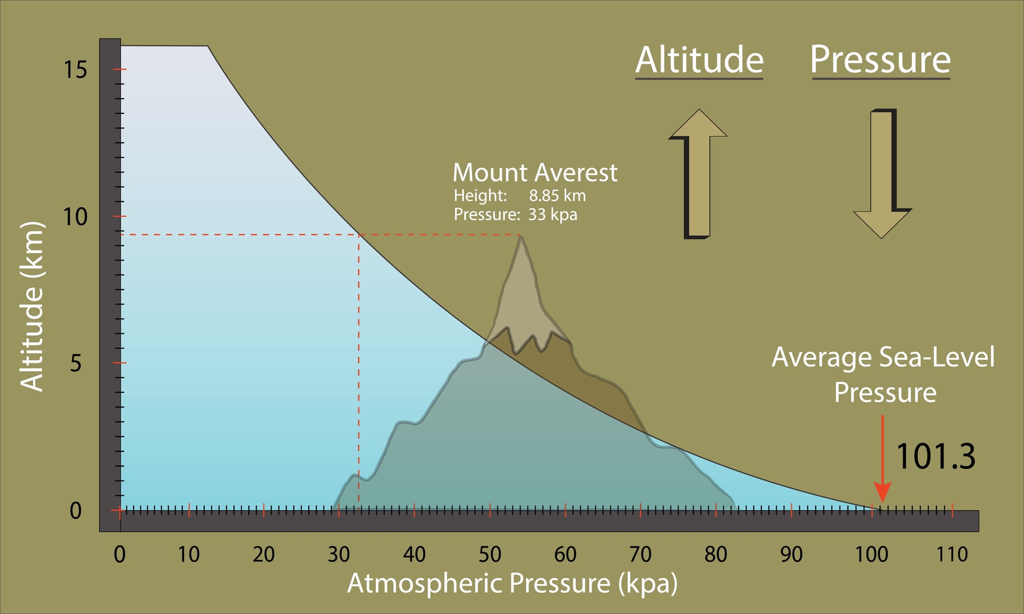
We can use the following formula to find the atmospheric pressure (which will be our surface pressure) as a function of altitude:
\(p_{surf}(h) = p_0 \cdot (1+\frac{Lh}{T_0})^{-\frac{gM}{RL}} \) \( p_{surf}(h): \text{Surface pressure at altitude h (in } Pascal) \) \( p_0: \text{Reference sea-level pressure } (p=101.325Pa) \) \( L: \text{Temperature lapse rate } L=0.0065K/m \text{ on average between 0-11km}) \) \( h: \text{altitude (in } m) \) \( T_0: \text{Sea level standart temperature } (T_0=288.15K) ) \) \( g: \text{Gravitational acceleration } (g\simeq 9.81m/s^2) ) \) \( M: \text{Molar mass of dry air } (M=0.02897kg/mol)\) \( R: \text{Univeral gas constant } (R\simeq 8.314J/(mol\cdot K))\)The idea, when building our pressure engine, is to initialize it by inputting the water density and the altitude, and then use it to calculate the pressure at any depth. Let's give it a try: let's try to calculate the ambient pressure at 20 meters (using a water density of 1025kg/m^3 and an altitude of 0m as parameters). Using our approximation, we would get :
\(P = D/10 + 1 \\ = 20/10 + 1 \\ = 2 + 1 = 3 bar\)And using our pressure Engine:
\(p(z) = \rho g z + p_{surf}(0) \\ = \rho g z + p_0 \cdot (1+\frac{Lh}{T_0})^{-\frac{gM}{RL}} \\ = 1025 \cdot 9.81 \cdot 20 + 101325 \cdot (1+\frac{0.0065\cdot 0}{288.15})^{-\frac{9.81\cdot 0.02897}{8.314\cdot 0.0065}} \\ = 201105 + 101325 \cdot(1+0)^{-5.2589} \\ = 201105 + 101325 \cdot 1 \\ = 302430 Pa \\ = 3.0243 bar\)As you can see, the approximation is really close to the value we got using our Engine; however, even these small differences do matter as they cumulate over time. To really illustrate how parameters can influence pressure, compute the pressure at a depth of 20 meters again, but this time, at an altitude of 1500m in a freshwater lake (meaning the water density is 1000kg/m^3):
\(p(z) = \rho g z + p_{surf}(1500) \\ = \rho g z + p_0 \cdot (1+\frac{Lh}{T_0})^{-\frac{gM}{RL}} \\ = 1000 \cdot 9.81 \cdot 20 + 101325 \cdot (1+\frac{0.0065\cdot 1500}{288.15})^{-\frac{9.81\cdot 0.02897}{8.314\cdot 0.0065}} \\ = 196200 + 101325 \cdot(1+0.0338)^{-5.2589} \\ = 196200 + 101325 \cdot 0.8396 \\ = 196200 + 85072 \\ = 281272 Pa \\ = 2.81272 bar\)Now, because we reduced the atmospheric pressure (surface pressure) due to the increase in altitude, and lowered the water density, our final computed pressure is lower, and our original approximation doesn't hold up as well. And this is why for a proper decompression planning tool, all of those parameters are extremely important to take into account.
And now that we're able to calculate pressure accurately, we'll be able to calculate the inert gas saturation pressure, tolerated ambient pressure at each depth, and all the rest!
Creating a compartment Model
There are many existing decompression models we could use in a planner. Most of them are available to the public (Bühlmann ZHL, DCIEM, RGBM, VVAL 18, etc...), but require an intricate comprehension of the theory and its specificity to implement properly. The easiest one to understand and implement - with the most documentation available- is surely the Bühlmann ZH-L model, and therefore, it is the one we'll talk about here. This model has many different variations, but the most common ones still used today are the ZH-L16B and the ZH-L16C.
The Bühlmann ZH-L16 models consider the human body to comprise 16 distinct compartments. These compartments vary from "fast" compartments to "slow" compartments, which describe the speed at which inert gas saturates and desaturates. To calculate the speed at which these compartments saturate/desaturate, we will use the concept of "half-time": a half-time is the time it takes for one compartment to be 50% saturated, after another half-time, it will be 75% saturated, then 87.5% saturated, and so on. The key point is that the diver (at any point) will be exposed to a certain ambient pressure, and every compartment will tend towards that pressure: if they start at a lower initial pressure, they saturate, and if they start at a higher initial pressure, they desaturate. For example, the following graphs shows how a a tissue with a half-time of 5 minutes would saturate and de-saturate:
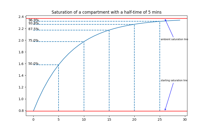
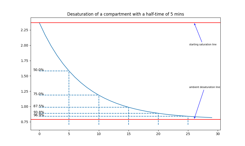
Click on the images to enlarge - a representation of saturation and desaturation in a compartment with a half-time of 5 minutes
If the diver is at a constant depth (meaning he doesn't change depths), breathing a certain mix, we can calculate the (de)saturation of a certain compartment using the following formula - also known as the Haldane formula:
\[P_{I,\text{ig}}(t_e) = P_{I,\text{ig}}(t_0) + (P_{gas,ig} - P_{I,\text{ig}}(t_0)) \cdot (1 - 2^{-t_e \over t_{I, 1/2}}) \quad \text{(Haldane)}\] \( P_{I,\text{ig}}(t_e): \text{Partial pressure of the inert gas dissolved in the compartment I} \\ \text{at the end of the exposure, expressed in bar} \) \(P_{I,\text{ig}}(t_0): \text{Partial pressure of the inert gas dissolved in the compartment I} \\ \text{before the exposure, expressed in bar} \) \(P_{gas,ig}: \text{Partial pressure of the inert gas in the breathing mix at ambient} \\ \text{pressure, expressed in bar} \) \(t_e: \text{duration of exposure, expressed in minutes}\) \(t_{I, 1/2}: \text{half time of the compartment I, expressed in minutes}\)If the diver is changing depth, but at a constant speed (during an ascent or descent), we can calculate the tissue pressure during the (de)saturation by introducing R, in the following formula - also known as the Schreiner formula:
\[P_{I,\text{ig}}(t_e) = P_{gas,ig} + R \cdot (t_e - {t_{I, 1/2} \over {\ln 2}}) - (P_{gas,ig} - P_{I,\text{ig}}(t_0) - {{R \cdot t_{I, 1/2}} \over {\ln 2}}) \cdot 2^{-t_e \over t_{I, 1/2}} \quad (Schreiner)\] \(R: \text{rate of change of the partial pressure of the inert gas in the} \\ \text{breathing mix, expressed in bar/min}\)For example, if a diver is ascending at 5m/min (~approximately 0.5 bar/min), breathing a mix containing 79% Nitrogen, then in this case, the R value for Nitrogen will be R=-0.5 bar/min × 0.79 = -0.385 bar/min. Notice the minus sign because during an ascent, we are reducing the pressure we are subjected to.
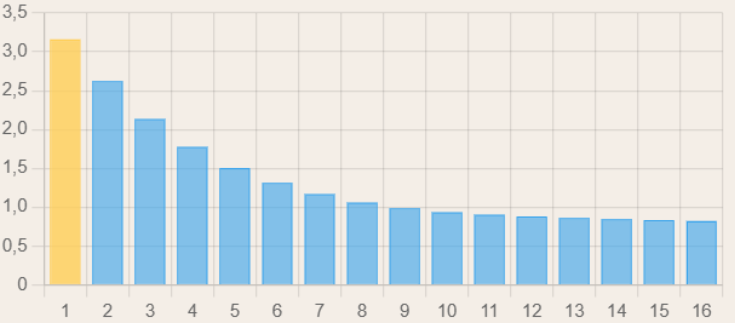
These two formulas are essential for our model: for each stop (be it a decompression stop, gas switch, the bottom phase, or anything else), and for every ascent/descent, the evolution of the dissolved inert gas pressure will have to be computed for each of the 16 compartments. Due to the different half-times, the fast compartments will saturate faster, and if we were to graph the saturation of our compartments after an initial saturation phase, it would look something like this (the leading compartment is marked in yellow):
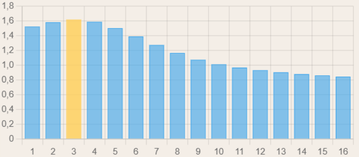
During the decompression phase, the faster compartments desaturate faster, meaning that one of the slower compartments becomes the leading one in terms of nitrogen saturation:
In any case, now that we understand how to calculate the inert gas pressure in our compartments, we can discuss the tolerated pressure, or the so-called m-values: the M-value of a compartment at a certain depth (M standing for "Maximum") is the maximum tolerated inert gas pressure this compartment can withstand before incurring high risks of DCS. This "M-value" is not fixed and varies as a function of the ambient pressure (the higher the ambient pressure, the more dissolved gas the body can handle) and also varies between compartments (fast compartments can handle a higher amount of dissolved gas compared to the slower ones). With Bühlmann's model, each compartment is assigned an a and b value, which can then be used to calculate its respective M-value using the following formula:
\[P_{I,\text{tol}} = {P_{amb} \over b} + a \quad (3)\]The a and b values can be found in the following table (these are the value for the C version of the model):
compartment |
1 | 2 | 3 | 4 | 5 | 6 | 7 | 8 | 9 | 10 | 11 | 12 | 13 | 14 | 15 | 16 |
|---|---|---|---|---|---|---|---|---|---|---|---|---|---|---|---|---|
half-time (min) Nitrogen |
5.0 | 8.0 | 12.5 | 18.5 | 27.0 | 38.3 | 54.3 | 77.0 | 109.0 | 146.0 | 187.0 | 239.0 | 305.0 | 390.0 | 498.0 | 635.0 |
a Nitrogen |
1.1696 | 1.0 | 0.8616 | 0.7562 | 0.62 | 0.5043 | 0.441 | 0.4 | 0.375 | 0.35 | 0.3295 | 0.3065 | 0.2835 | 0.261 | 0.248 | 0.2327 |
b Nitrogen |
0.5578 | 0.6514 | 0.7222 | 0.7825 | 0.8126 | 0.8434 | 0.8693 | 0.8910 | 0.9092 | 0.9222 | 0.9319 | 0.9403 | 0.9477 | 0.9544 | 0.9602 | 0.9653 |
half-time (min) Helium |
1.88 | 3.02 | 4.72 | 6.99 | 10.21 | 14.48 | 20.53 | 29.11 | 41.20 | 55.19 | 70.69 | 90.34 | 115.29 | 147.45 | 188.24 | 240.03 |
a Helium |
1.6189 | 1.383 | 1.1919 | 1.0458 | 0.922 | 0.8205 | 0.7305 | 0.6502 | 0.595 | 0.5545 | 0.5333 | 0.5189 | 0.5181 | 0.5176 | 0.5172 | 0.5119 |
b Helium |
0.4770 | 0.5747 | 0.6527 | 0.7223 | 0.7582 | 0.7957 | 0.8279 | 0.8553 | 0.8757 | 0.8903 | 0.8997 | 0.9073 | 0.9122 | 0.9171 | 0.9217 | 0.9267 |
Notice that there are different values for helium and nitrogen. If helium is present in the mix, the saturation/desaturation must be calculated independently of the nitrogen. As for the tolerated pressure, instead of calculating it two times, the total dissolved inert gas in the body must be considered (PN2 + PHe), and the Ptol should be calculated using a weighted average of the a and b values for Nitrogen and Helium. More specifically, for each compartment, we can use:
\[a = \frac{a_{N_2}\cdot p_{N_2} + a_{He}\cdot p_{He}}{p_{N_2}+ p_{He}}\] \[b = \frac{b_{N_2}\cdot p_{N_2} + b_{He}\cdot p_{He}}{p_{N_2}+ p_{He}}\]Ok. So now, we know how to calculate the dissolved inert gas in our body by using compartments, and we know how to calculate the maximum tolerated amount of that inert gas for each compartment as a function of the ambient pressure. But before using all those, there is one last thing we will need to talk about: gradient factors.
Gradient factors are tools to quantify how far we would like to "stay away" from this tolerated pressure - simply said, the gradient factors allow us to control the conservatism of the dive plan. Although this article's purpose isn't to explain gradient factors in depth, but rather how to use them, I will still go over the basics quickly.
Gradient factors consist of a number pair: GF LOW and GF HIGH, usually represented as X/X (for example, a conservatism of 40/80 means the user chose a GF LOW of 40, and a GF HIGH of 80). These numbers represent the percentage of "how close" our decompression planner will get us to the tolerated pressure compared to the ambient pressure in the leading compartment (the leading compartment is the one that is closest to the so-called M-value). The GF Low will dictate at what percentage of the M-value the first decompression stop will generate, while the GF High will dictate at what percentage of the surface M-value the diver will be allowed to finish their decompression and finally surface. The Gradient factors act as a ramp: this means that between the depth where the first decompression stop is generated and the surface, the GF ramp will assume all values between GF Low and GF High. To give an example, if a diver chose Gradient Factors of 40/80, and their first decompression stop would be generated at 21m, then the stops at the following depths: 18, 15, 12, 9, 6, and 3 meters would all respectively assume the following gradient factors: 46%, 52%, 58%, 64%, 70%, and 76% (roughly).
This percentage is relative to the ambient pressure. For a more visual approach, observe the graph below: The diver starts at the red cross (bottom right) and slowly ascends (moves to the left of the graph, reducing his depth), and as soon as he hits the "gradient factor line", stops are generated until his saturation lowered enough to move to the next stop.
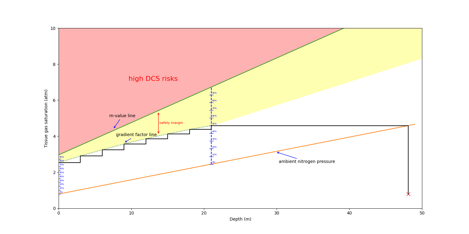
As mentioned above, we will have to verify for each ascent step that all 16 compartments don't exceed their gradient factor line. As we'll see later in the decompression algorithm, we will have to actively look for the depth of our first decompression stop using the GF Low value to actually be able to get our gradient factor line.
Creating a diving grid
Now that we have the tools to understand and model how dissolved inert gases behave in our body, the next part of building a decompression planner is going to be finding a way to enable the planner to use this model to create a pathway to actually generate a decompression plan. The way we chose to do this is by starting to create a "depth" grid from the bottom plan the user input. This means that we will generate a grid of all the possible depths the diver might have to go through to complete their decompression.
As the most common depths to decompress are multiples of 3s (6m, 9m, 12m, etc...), we will add each multiple of 3 present between whichever depth(s) the diver plans to go to and the surface. For example, if the user wants to go to a depth of 40 meters, regardless of the gas he breathes, and the time he spends there, his decompression stops will have to fit the following grid: [40, 39, 36, 33, 30, 27, 24, 21, 18, 15, 12, 9, 6, 3]. For the sake of simplifying the decompression planner's task, we will also include the start and end depth (which is 0m) in the grid [0, 40, 39, 36, 33, 30, 27, 24, 21, 18, 15, 12, 9, 6, 3, 0] as this tells the decompression planner that the diver starts from the surface and ends at the surface. Notice that the grid between 0m and 40m is not present: this is deliberate, as there is no need to decompress when descending; however, when ascending, there might be a necessity to perform a decompression stop. This "depth grid" also works perfectly when the diver wants to plan a multi-level dive: for instance, assume that a diver wants to plan a dive where he will go to 20m, then shallow up to 10m, before going back down to 30m. The generated depth grid would then be: [0, 20, 18, 15, 12, 10, 30, 27, 24, 21, 18, 15, 12, 9, 6, 3, 0]. As a sidenote, it is important that if the diver adds a multiple of 3 in the plan, the grid generates it again, as there might be some additional decompression required at this depth using a different gas (for example, if a diver plans a multi-level dive at 20m and 12m, 12m must appear twice: [0, 20, 18, 15, 12, 12, 9, 6, 3, 0]). This "grid system" is very convenient as it is extremely easy to tweak: for example, by removing the last 3m or adding an intermediate 4.5m, we can choose at which depth the last stop will be, or we can even choose to decompress at depths which are multiples of 2 instead of 3 (or whichever other pattern we choose).
Before moving on to the actual implementation of the decompression algorithm, we will need to expand this "grid" a little bit: we have the depths the diver will go through (in the final decompression plan, the depths the diver spends no time at will be removed from the plan), but there is still more information we need to add. When the user inputs their plan, the information we get is:
- The time he wants to spend at each planned depth
- The gas used at each planned depth
- The decompression gases available
Using this information, we want to expand the "depth grid" to get a grid where each depth has the time spent there and the gas used. For the depths which were added as part of the grid, the time will by default be 0, but will be increased if the model that a decompression stop is necessary (more information on that later, as it will be part of the main decompression algorithm), as for the gas, we can already know will be the best to use at each depth (also more information about this in the next section).
To give a concrete example, imagine a diver plans a multi-level dive where he spends 20 minutes at 40 meters using an EAN 28 blend, followed by 10 minutes at 20 meters using that same EAN 28 blend, and he also has an EAN 50 blend available as a decompression gas. The final grid we would want to obtain is:
- 0m, 0min, EAN 28
- 40m, 20min, EAN 28
- 39m, 0min, EAN 28
- 36m, 0min, EAN 28
- 33m, 0min, EAN 28
- 30m, 0min, EAN 28
- 27m, 0min, EAN 28
- 24m, 0min, EAN 28
- 21m, 0min, EAN 50
- 20m, 10min, EAN 28
- 18m, 0min, EAN 50
- 15m, 0min, EAN 50
- 12m, 0min, EAN 50
- 9m, 0min, EAN 50
- 6m, 0min, EAN 50
- 3m, 0min, EAN 50
- 0m, 0min, EAN 50
This is as much information as we can provide to the decompression model before we let it do its thing. But before looking at that, let's talk about how the optimal gas is chosen.
Choosing the right gas for the right depth
Picking the gas blend that fits the decompression stop optimally is a question of choice in the diving plan and the model: this means that there are different ways to "choose conditions" to choose our gas. For example, the most straightforward condition to implement would be: At a certain depth, exclude the gases whose ppO2 is outside the safe range (usually 0.18-1.6 bar), then, out of the available gases, select the one with the highest ppO2. Although at first, this condition can seem reasonable to maximize off-gassing, it will lead to potential issues for deeper dives, where a switch to a travel gas will happen too deep. To avoid this, one of the solutions is to implement a "max Equivalent Narcotic Depth" for a deco mix. This means that if the END of a gas mix is deeper than a chosen limit, the mix will be excluded from the selection at this particular depth. To integrate this process seamlessly, we recommend letting the user choose the max Equivalent Narcotic Depth (while limiting its value to avoid absurd entries) and also allowing them to choose their preferred max ppO2 for decompression (some may prefer to switch at 1.3, 1.4 or 1.5 ppO2 rather than 1.6 bar). Some other options for the user might include the choice to either switch at the MOD or to switch at the first decompression stop (although both may sometimes coincide, it is not the same thing).
Another issue to deal with when choosing gases for multiple depths is the risk of Isobaric Counterdiffusion (ICD) during a switch (due to the sudden change of helium/nitrogen fraction). There are two main ways around this: the first solution is to allow the decompression model to choose the gas that minimizes this risk, but then it becomes a question of cost-tradeoff "which gas has the most optimal ppO2, lowest END, and lowest risk of ICD, and if it's a mix, which of those conditions becomes the most important one?" - although this solution is not impossible to implement, but it is certainly not easy. The second solution, which is more pragmatic, is to ignore ICD during the switch condition, but to give an alert to the user when there is a high ICD risk. This will allow the diver to adjust the mixes accordingly before validating the plan. As for the condition triggering an ICD alert, we chose to follow the "rule of fifth" (which is more a rule of thumb than an actual rule), which states that the increase of the Nitrogen fraction should be lower than one-fifth of the decrease of the Helium fraction.
The decompression algorithm
Everything we have talked about previously is the prerequisite for being able to run the decompression algorithm properly. Now let's get straight into it: the idea behind the algorithm is that we have the depth grid we previously generated, and we want to know which stop we have to complete to safely go from the start to the end of the grid (start from the surface, complete the dive plan, and end back at the surface). To do that, we will repeat the following steps, starting at the first step of the grid:
- Calculate the new nitrogen/helium saturation of our tissues given our exposure time at that stop using the Haldane formula (if the exposure time is 0, the formula won't change the saturation level of the tissues).
- Before going to the next step's depth, calculate the saturation of each tissue after the ascent/descent to travel to the next stop, using Shreiner's equation.
- At this new step, calculate the M-value for all compartments using the current saturation level. Make sure to multiply each compartment's M-value by the gradient factor (if the depth of the first decompression stop has not been found yet, use the value of the GF Low; if it has been found, adjust the gradient factor value accordingly)
- For each compartment, compare the adjusted M-value to its respective dissolved inert gas partial pressure. If all of the compartment partial pressures are below their adjusted M-value, the ascent is allowed (Go to step 6). If ANY of the compartments exceed their adjusted M-value, the ascent isn't allowed (Go to step 5).
- If the ascent isn't allowed: go back to step one with the previous step of the grid (undo the saturation that was calculated for the ascent/descent using Shreiner's equation, as if we "never moved" from the previous stop), but add a unit of time (1 minute, for example) to the stop time: this will be a decompression stop.
- If the ascent is allowed: start again from step one, with the next step of the grid.
In simpler terms, what this algorithm does is verify if any decompression is required at each step before moving on to the next step of the grid. This is why in the previous section, we mentioned that we would add the first and last 0 as the algorithm must check the last decompression stop to ensure going back to the surface is allowed. The algorithm also operates on the descent/bottom part of the plan, but as the M-values are way larger than the value of the tissue saturation, no required decompression is found there.
The result of this algorithm will be a grid with new time values, with the appended times at depths where decompression was required to move on to the next step. To return a readable and user-friendly version to the user of the decompression planner, we can remove all the steps where the time value is still 0 (as nothing happens at those depths). Additionally, we can also insert intermediate steps, which give information about ascents/descents and gas switches where they take place.
Final report
Finally, now that we have the decompression plan, we can run through it and calculate everything that is needed to give an extensive report about the dive itself. This would include:
- Total gas requirements
- Total Oxygen Toxicity Units (OTUs) accumulated
- Single-dive CNS %
- Daily CNS%
Let's have a quick overview of how each of those can be calculated.
Gas consumption
To calculate gas consumption, the user must provide their SAC rate. There is usually a different breathing rate for the bottom part of the dive and the decompression phase. Using the SAC rate to calculate total gas consumption is pretty straightforward: the SAC rate represents how many Liters per Min the diver breathes on the surface; therefore, to find how much they breathe at a certain depth for a certain duration, simply multiply the SAC rate by the time spent at that depth and the ambient pressure:
\[V_{used}=SAC\cdot t \cdot p_{amb}\]The used gas should be calculated individually for every step of the dive plan, and added together for the same gases at the end: for the steps with a constant depth (bottom stops and decompression stops), this is quite straightforward, but for ascents/descents, the average depth over the duration of the movement should be used.
Small Note about Gas consumption: when referring to consumed gas, a lot of people are going to talk about "Liters", the correct unit for the unit of gas is actually the "bar Liter".
OTUs
OTUs are tracked as a means of limiting exposure to increased oxygen partial to avoid pulmonary & occular oxygen toxicity. A diver subjected to one atmosphere of Oxygen partial pressure will accumulate one OTU, but the accumulation per minute can vary as ppO2 varies. To calculate total OTUs, calculate OTUs for each step, and add up the total of all steps together. For each step, the ppO2 must be calculated, and you must multiply the exposure time to the OTU/min value using the following table:
| ppO2 (bar) | OTUs/Min |
|---|---|
| 0.5 | 0.00 |
| 0.6 | 0.27 |
| 0.7 | 0.47 |
| 0.8 | 0.65 |
| 0.9 | 0.83 |
| 1.0 | 1.00 |
| 1.1 | 1.16 |
| 1.2 | 1.32 |
| 1.3 | 1.48 |
| 1.4 | 1.63 |
| 1.5 | 1.78 |
| 1.6 | 1.92 |
| 1.7 | 2.07 |
| 1.8 | 2.21 |
CNS single & daily limit
The CNS% helps us avoid CNS Oxygen toxicity. There is both a single-dive exposure and a daily exposure CNS value to track. Both CNS values, similar to the previous values, must be calculated at each step and summed at the end. To do that, start by calculating the ppO2 at each step, and refer to the following table for the time limit.
| ppO2(bar) | CNS single-dive limit (min) | CNS daily limit (min) |
|---|---|---|
| 1.6 | 45 | 150 |
| 1.5 | 120 | 180 |
| 1.4 | 150 | 180 |
| 1.3 | 180 | 210 |
| 1.2 | 210 | 240 |
| 1.1 | 240 | 270 |
| 1.0 | 300 | 300 |
| 0.9 | 360 | 360 |
| 0.8 | 450 | 450 |
| 0.7 | 570 | 570 |
| 0.6 | 720 | 720 |
Then, using the time spent at this depth, calculate the percentage of the CNS accumulated using:
\[CNS_{single}=\frac{t}{t_{limit,single}}\times 100\] \[CNS_{daily}=\frac{t}{t_{limit,daily}}\times 100\]Finally, add up all the calculated CNS% values to get the total percentage for single and daily limit.